- Articles
- Borland C++ Sorting Algorithm
Jul 7, 2014 (last update: Jul 7, 2014)
Borland C++ Sorting Algorithm
Score: 4.3/5 (110 votes)
INTRODUCTION
Have you ever wondered about the software programs that sort large numbers of items? We take them for granted to do our everyday tasks on the computer, but what exactly makes them function? Many software packages have implemented their own algorithms for taking care of this job. I have developed my own approach for handling this important task and I will present a detailed explanation here of how it works.
AN OVERVIEW OF MY PROBLEM
In 1996 I was working on an inventory system for a customer using procedural C programming to sort a large number of items - about 8,000 to 10,000. The sorting program I had at the time was something I created in the early 1990s and could only sort up to 1,500 items. This Borland C alphabetizing code is listed on my website.
Back in the mid 1990s, most IBM PC based computers were running Intel 486, Intel Pentium, AMD K-5, etc. However, their capability and that of the hard disks at the time seemed like they had to struggle to handle a large capacity sorting task like the one my application required. I had to start with the basic programming idea behind my procedural C sorting code from the early 1990s and somehow expand it so it could process larger data files. If I tried to design the new sorting program so it did most of the work on the mechanical hard disk that would have created a new problem. Attempting to sort a large data file on a disk drive would have created a very big reduction in speed because of slowness of the mechanical moving parts of the hard disk. The customer would certainly object to the slower speed and I would have been sent back to the drawing board to start over with something more acceptable.
Performing the sorting on the hard disk was obviously a road to nowhere with a large data file. The only other option I could think of was to do the bulk of the work in the memory. By concentrating the data manipulation in memory, I could escape the slower world of the mechanical disk drive and pick up much more speed. This was especially important at the time because of the less powerful processors of the day. Another compelling reason for shifting the work into memory was because doing much of the work on a disk that could potentially have any number of sector errors on it could create catastrophic problems. This would have thrown a wrench into the sorting process and created a corrupted output file. Of course this is also possible with concentrating the work in memory, but it’s less likely to occur.
MOVING FORWARD
I will begin discussing the “nuts and bolts” of how my algorithm works shortly. This new and improved alphabetizing code for sorting jobs was later adapted to Borland C++ and I have included pieces of the code along with diagrams to help illustrate the logic flow. Please note that some of the C++ variables are referred to as “non-persistent” variables, while the “top” and “bott” variables are called “persistent” variables. This is because “non-persistent” variables are completely reset to new values during the processing while “persistent” variables are incremented or decremented at various times, but never reset. Also, you will notice I refer to various data structures I use such as “grid”, “name”, and “stor” as conventional data structures. They are allocated within the boundaries of the 64K data segment as prescribed by the small memory model I used in the programming. This is to differentiate them from the far memory data structures “s”, “s1” and “s2”. This algorithm was performed on binary fixed width text files. I use these in my application development because they are easy to work with. The algorithm can easily be adjusted to work with binary variable width (delimited) text files, also.
THE MAIN OBJECTIVE: LARGER SORTING CAPACITY
Now that I had decided to focus most of the processing in the memory, I had to come up with a way to do this so it could allocate the capacity for a large number of items. In Borland C/C++, there were 6 memory models to choose from: tiny, small, medium, compact, large and huge. I always used the small memory model since it was the default and I just became accustomed to dealing with it since I started with C coding in 1990. In the small memory model, the code and data segments each have 64K of memory available. In order to sort large numbers of items, I would need a much larger space of memory than a 64K data segment that also had to hold a variety of other data structures.
I decided to use the far side of the heap, or what is known as “far memory”. To set this up, I first included a necessary C++ header file for allocating far memory:
Then I declared 3 far memory pointers like this near the beginning of the sorting code:
I allocated them like this to handle up to 16,000 items:
The reason I set up 3 far memory data structures is because all of them are needed to manipulate the data with the new sorting algorithm I created. This gave me the space to manipulate up to 16,000 items. I could have allocated for a larger number of data records, but this was more than enough to do the job at hand.
ASSIGNING A NUMERICAL WEIGHT TO EACH ITEM IN THE DATA FILE
The processing starts with applying a mathematical formula to the first four characters of each item in the binary fixed width text file. Consider the following numerical succession of powers of “10”:
10,000,000 1,000,000 100,000 10,000 1,000 100 10 1
Next, remove the following powers of “10” in the above numerical succession:
1,000,000
10,000
100
10
This is what is left with these powers of “10” in the updated numerical succession:
10,000,000 100,000 1,000 1
The ASCII codes of each character in a given item can range from 32 to 126. Each of these ASCII codes has been “mapped” to numerical values ranging from 0 to 94. The numerical values for each of the first four characters starting from the beginning in a given item will each be multiplied by the updated numerical succession in a left to right fashion.
This is the math formula I use in the programming to assign numerical weights to each item:
(10,000,000 X numerical value of character 1) +
(100,000 X numerical value of character 2) +
(1,000 X numerical value of character 3) +
(1 X numerical value of character 4)
This amount is equal to the numerical weight for this item. Consider the following example:
"SMITHSON"
"S" = Character 1
"M" = Character 2
"I" = Character 3
"T" = Character 4
"H" = Character 5
"S" = Character 6
"O" = Character 7
"N" = Character 8
ASCII code for Character 1: S = 83 which corresponds to numerical value 51 per the algorithm.
ASCII code for Character 2: M = 77 which corresponds to numerical value 45 per the algorithm.
ASCII code for Character 3: I = 73 which corresponds to numerical value 41 per the algorithm.
ASCII code for Character 4: T = 84 which corresponds to numerical value 52 per the algorithm.
Now, let’s plug in the numerical values from this example to the math formula to yield the numerical weight for the above item:
(10,000,000 X 51) + (100,000 X 45) + (1,000 X 41) + (1 X 52) = 514,541,052
This math formula is something I came up with that I believed would be a good way to assign a numerical weight to each item. Here is a partial piece of the code that performs this task in the program:
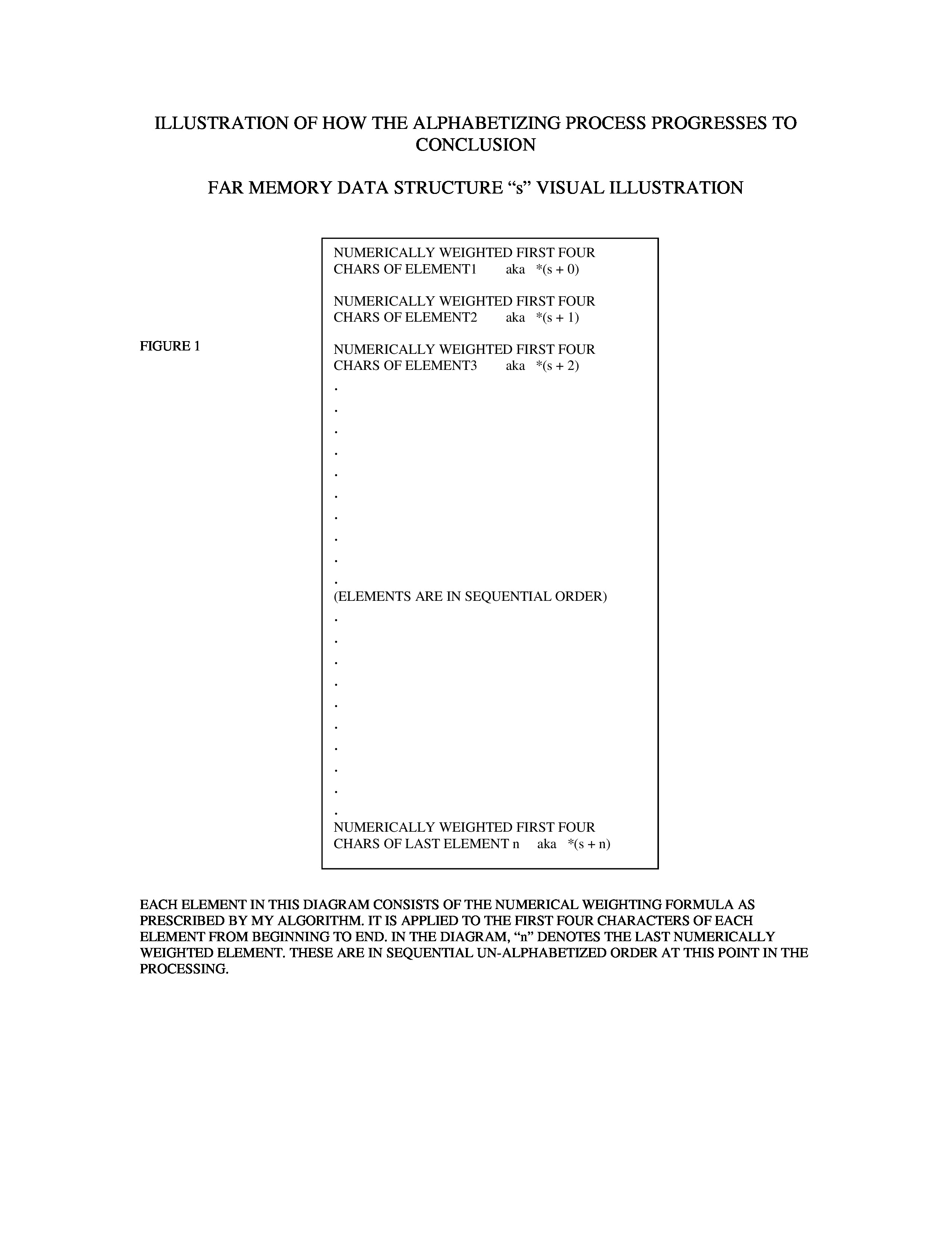
The lowest and highest numerical weights are now known after we have applied this math formula to all the items in the data file. All numerical weights will be stored in the far memory data structure “s” in positions that correspond to their sequential positions in the unsorted data file (See Figure 1).
In the above patch of code, the first thing that occurs is to see whether or not the lowest and highest numerical weights are equal. This compares the lowest primary variable “low1” to the highest primary variable “up1”. If they are equal, the start of processing will be aborted because all items will have the same numerical weight. This means the first 4 characters of all items are the same. This would be highly unusual because they would already be nearly sorted to begin with and the probability of ever encountering a data file like this would be remote. In the end, the original data file to be sorted would be left intact and not be reconstructed at the end. If they are unequal, the lowest primary variable “low1” and the highest primary variable “up1” would represent two different sets of numerically weighted items and therefore processing would continue with the commencement of the “main” processing loop.
A TALE OF TWO FAR MEMORY PROCESSING REGIONS: “TOP1” AND “BOTT1”
The program cycles around a “do-while loop” which I call the “main” processing loop. I use 2 regions of far memory to facilitate the sorting process, which I call the “top1” and “bott1” processing regions. Each of these will be repeatedly redefined with each loop through the “main” processing loop. This is the “segmented mechanism” which drives the sorting process.
Both of these processing regions actually begin as numerical variables. They later evolve into processing regions. First, they are both initialized to 0. Then “top1” is incremented by 1 for each item in the far memory data structure “s” that corresponds to the lowest primary variable, “low1” (lowest current numerical weight). Next, “bott1” is incremented by 1 for each item in the far memory data structure “s” that corresponds to the highest primary variable, “up1” (highest current numerical weight). This is done in the above code. Also, the “main” processing loop exit variables “qqq” and “sss” cannot be set to exit the “main” processing loop while both processing regions need to be redefined to process unsorted items. In other words, “qqq” must be set to 0 for “top1” to include the lowest current numerical weight in its processing region that is being defined. And “sss” must be set to 0 for “bott1” to include the highest current numerical weight in its processing region, which is also being defined.
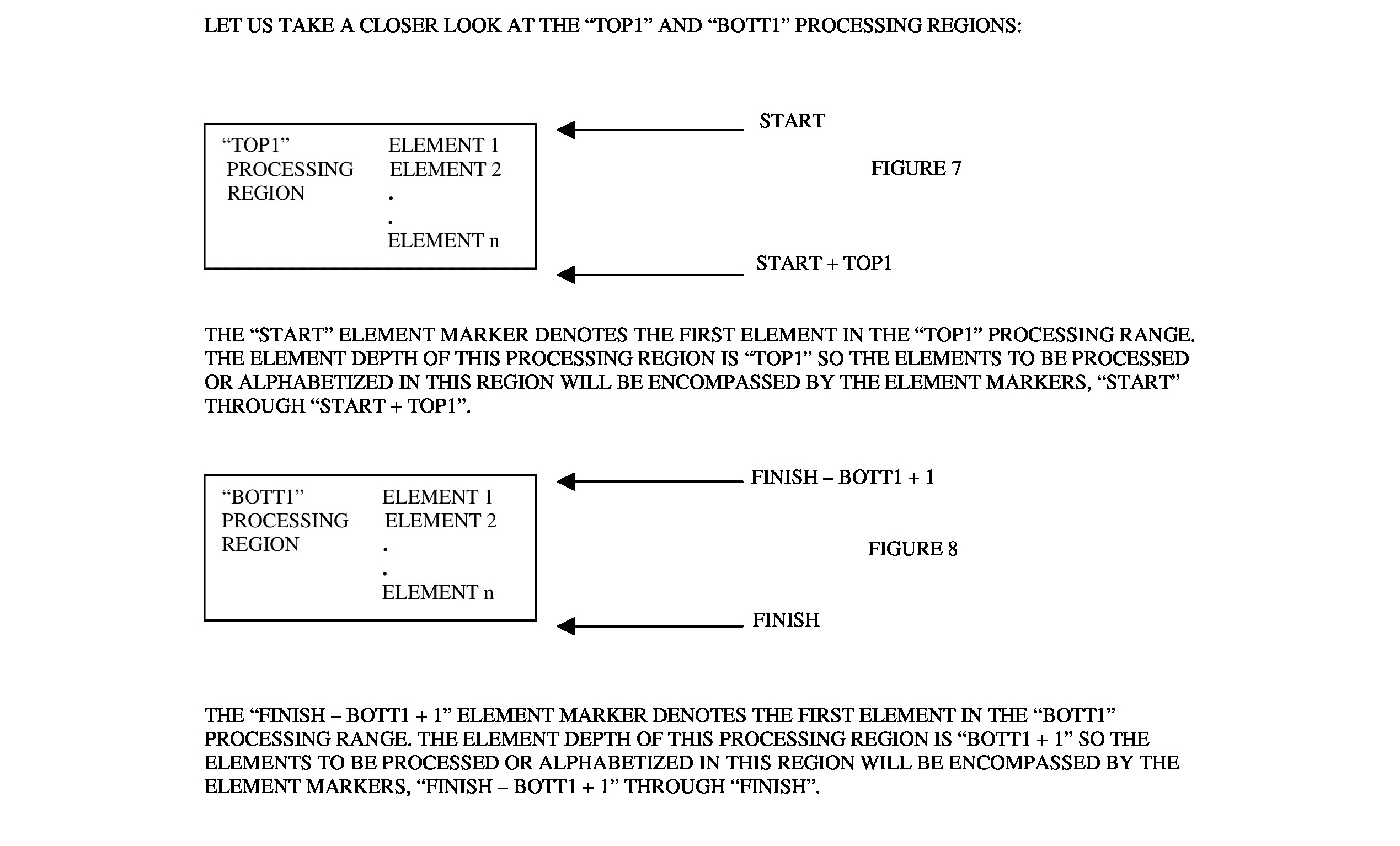
One other thing to notice in the previous code are 2 markers I use for the items denoted by “start” and “finish”. “start” is assigned the value in “top”, and “finish” is assigned the value in “bott”. “start” is a “non-persistent” item marker used to denote the item count or depth of the “top1” processing region. “finish” is a “non-persistent” item marker used to denote the item count or depth of the “bott1” processing region. Both “top” and “bott” are “persistent” item markers that are incremented along with “top1” and “bott1”. (See Figures 7 and 8 to see a visual representation of the “top1” and “bott1” processing regions.)
After the redefinition process is completed, the “top1” processing region will encompass items corresponding to the lowest current numerical weight. The same is true for the “bott1” processing region, but with a numerical weight that corresponds to the highest current numerical weight. The algorithm will use both processing regions to facilitate the actual sorting process, the specifics of which I will not get into with this article. To view that, you can refer to the “improved alphabetizing code” hyperlink near the beginning of the article. After the sorting has been performed, the program will loop around the “main” processing loop and proceed to redefine new pairs of “top1” and “bott1” processing regions. (See Figure 2).
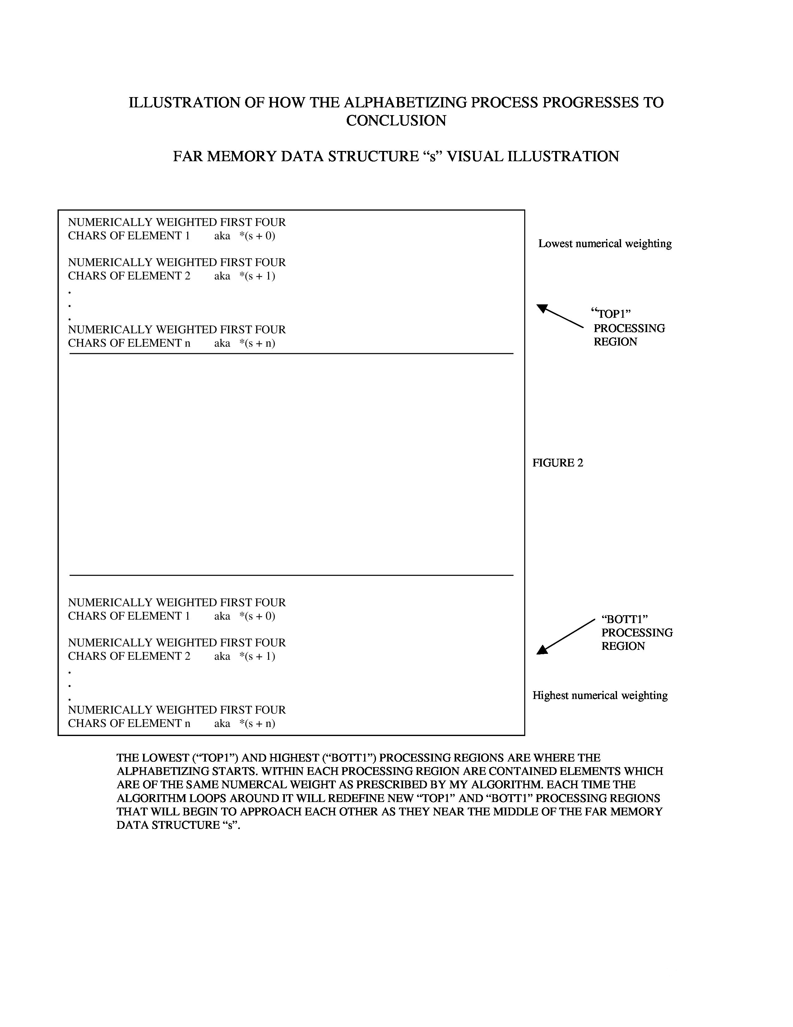
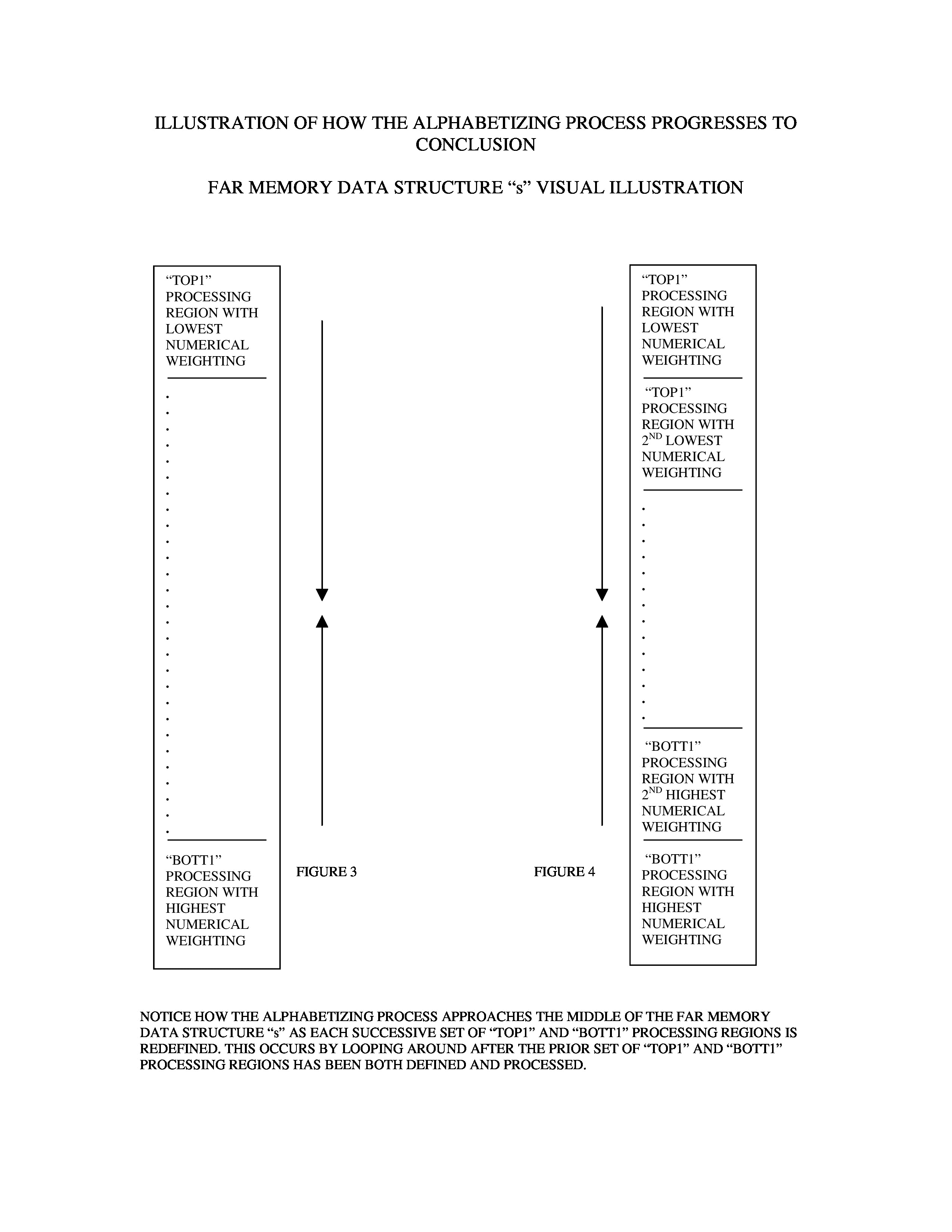
Both processing regions will approach each other in spatial proximity as they move toward the center of the far memory data structure “s” from being redefined with each pass through the “main” processing loop. Each new “top1” processing region will have a higher numerical weight than its predecessor “top1” region. Each new “bott1” processing region will have a lower numerical weight than its predecessor “bott1” region. Please refer to figures 3, 4, 5, and 6 for a visual illustration of the progression of the algorithm as successive “top1” and “bott1” processing regions are redefined with each pass through the “main” processing loop.
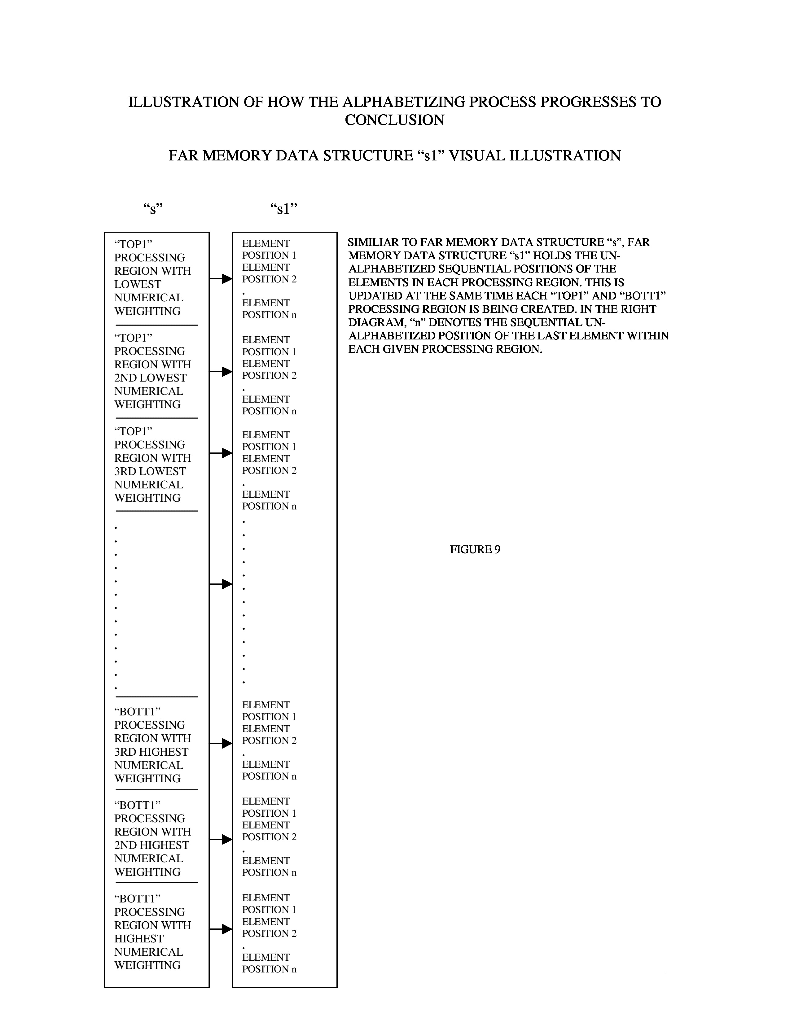
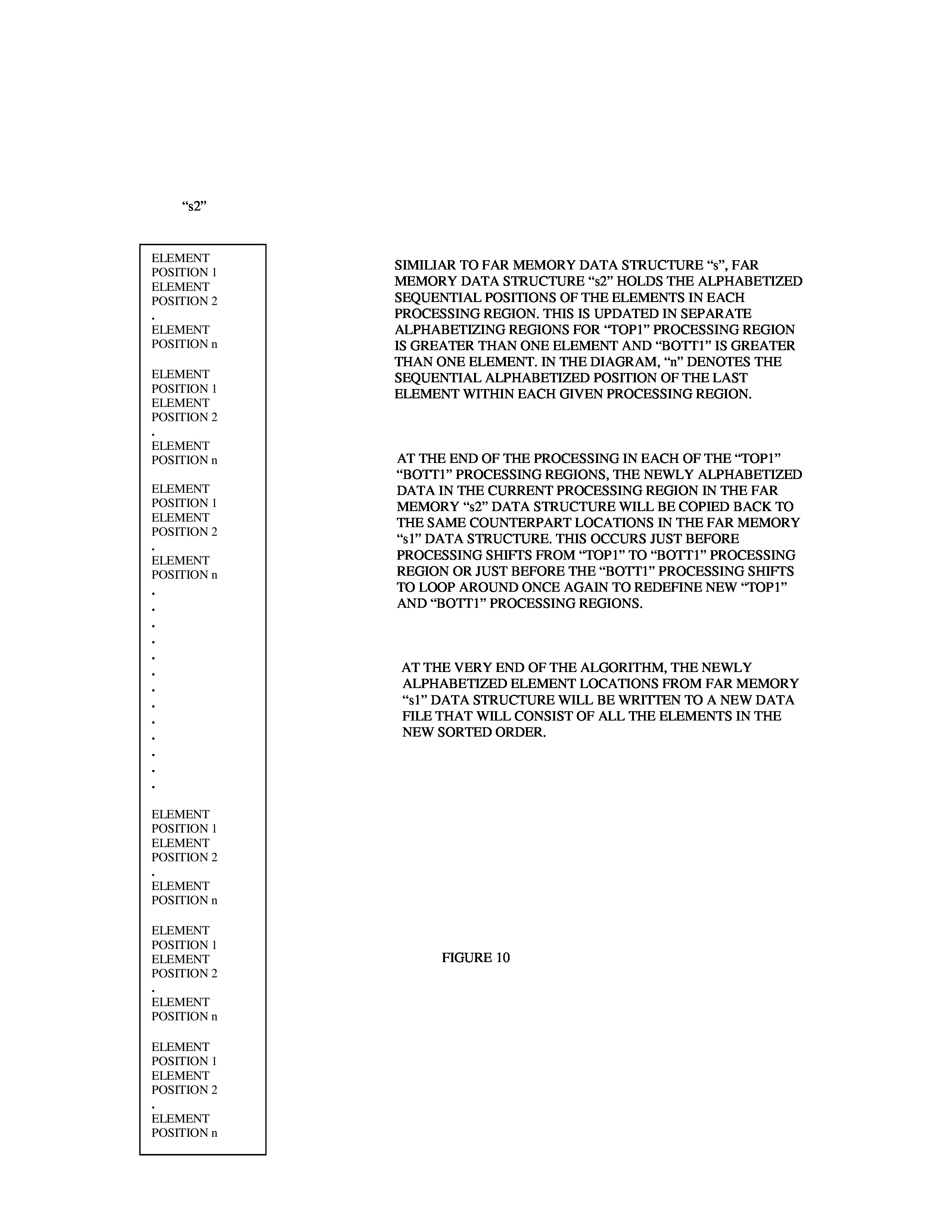
Notice what happens in Figure 6 after the processing in successive “top1” and “bott1” processing regions reaches the middle of far memory in the far memory data structure “s”. The “top1” processing region with the least lowest numerical weight is adjacent to the “bott1” processing region with the least highest numerical weight. The processing will cease at this point because there will be no more items left to sort. The “main” processing loop will then be exited and the new sorted array of item positions stored in far memory data structure “s1” will be written to a new data file. (See Figures 9 and 10).
Here, I want to talk about ways the “main” processing loop could be exited before the data is written back to a newly sorted data file. As the processing draws to a close in the middle of the far memory data structure “s”, it will not necessarily end with an even pair of final “top1” and “bott1” processing regions. It can also near completion with either of the “top1” or “bott1” processing regions having its “main” processing loop exit variable set to attempt to exit the “main” processing loop. To be more specific, the “top1” processing region could have its “main” loop exit variable “qqq” set to 1, which means there are no more “top1” regions to be redefined. The “bott1” processing region could have its “main” loop exit variable “sss” set to 0, meaning there is another “bott1” processing region to be redefined and sorted. The opposite of this can also occur.
AN ANALOGY THAT MAY HELP CLARIFY THE LOGIC FLOW
Knowing this narrative may be overwhelming for some readers, I would like to take a page from American history that may be helpful in creating a better understanding of how my algorithm works.
During the latter part of the 19th century, the United States turned its attention to nation building. Connecting the vast expanse of North America by way of a coast-to-coast railroad became a national priority. This was the start of America’s first Transcontinental Railroad.
Two railroad companies, the Union Pacific and the Central Pacific, spearheaded this ambitious and daunting task. The Central Pacific began building its railway eastward from Sacramento, California, while the Union Pacific began construction work heading westward from Omaha, Nebraska.
Both crews in the east and west worked relentlessly for seven years. On April 28, 1868 the Union Pacific’s construction gang of Chinese and Irish workers laid ten miles of railroad track in a single day as a result of a $10,000 bet that it could actually be done. On May 10, 1869 the construction was completed at Promontory Point in the Utah territory. The Union Pacific’s No. 119 engine and the Central Pacific’s No. 60 engine, Jupiter, were drawn up face-to-face separated by the width of a single railroad tie. At the Golden Spike ceremony, three spikes were driven in to connect the two railways: gold, silver and a composite spike made from gold, silver and iron. Travel time between the east and west coasts of the United States was reduced from 4 to 6 months to only 6 days by railroad!
Now, the progression of my algorithm is quite similar to the construction of America’s first Transcontinental Railroad when you take a moment to really think about it. As the algorithm moves along, it begins to resemble two work crews gradually progressing towards a conclusion in the middle of the allocated far memory space, which is like a long stretch of terrain awaiting the arrival of “sorting construction labor”, so to speak. The “top1” and “bott1” processing regions are like “two construction gangs” that commence “sorting work” that begins at opposite ends of the allocated memory space. They each work hard to sort items of the same numerical weight as previously described, while constantaly moving closer and closer to one another. After the program loops around the “main” processing loop and new “top1” and “bott1” processing regions have been defined, the process repeats itself. Finally, The “Golden Spike Ceremony” occurs when the “top1” and “bott1” processing regions are adjacent to one another somewhere near the middle of the allocated far memory segment - Promontory Point in the Utah territory, if I may use that to hopefully foster a better understanding of my algorithm.
A POTENTIAL PROBLEM AND A REMEDY
Here, I would like to expand on a potential problem with my algorithm and a recommended solution that should take care of it. The 2 dimensional “grid” conventional data structure is used extensively to manipulate items in the “top1” and “bott1” processing regions. It is designed to hold up to 150 items of the same numerical weight. You need to be conscious about how much row depth you give the 2 dimensional “grid” conventional data structure so it and other conventional data structures taken together don’t breach the 64K data segment of the small memory model that is used. The problem arises if there are more than 150 items in a “top1” or “bott1” processing region. The algorithm won’t abort or malfunction, but rather it will include only the first 150 items in a processing region. I never really tried to address this potential snafu, because it is highly unlikely to occur in the first place. There would have to be more than 150 “Smiths” or “Joneses” to trigger the glitch. This could potentially happen in a voter registration verification data file that could include a large number of same last names.
A good way to correct this is to declare a fourth far memory data structure of the same size as each of the first 3. It would replace and perform the job of the 2 dimensional “grid” conventional data structure, yet it would always be large enough to hold all the items for a particular numerical weight. This is because it would be allocated to hold as many items as are in the entire data file.
JUST SAY “NO” TO REDUNDANT, SPEED ROBBING CODE
Many of you may be wondering by now about the speed of the algorithm. I tested it with a binary fixed record width text file containing 10,959 part numbers. On a Gateway Pentium 4 tower CPU using an old 6 GB Quantum Bigfoot hard drive the processing took a little over 3 seconds. When it was run on a Dell M5030 laptop with an AMD V160 Processor at 2.4 GHz it took about 1 second. There are some areas in the “do-while” loop processing that could be redesigned or eliminated that should further increase the processing speed since less work is required to achieve the same result. After I finished this in 1996 it seemed to work in a reasonable amount of time so I didn’t go back and try to optimize it some more. Here I will elaborate with some selected areas in the code that could be improved to yield more processing speed.
This block of code that tests for ASCII characters 32 through 126 could be replaced with the C++ function, “atoi()”. It would eliminate much of the repetitive conditional “if-then” logic structure comparisons and convert the character to an integer. This new integer value could then be used in the math formula that computes numerical weights for each item. Here is another place for adding some speed:
In the “top1” and “bott1” processing sections of the code, there is a patch of code enclosed by processing loop “2”. There are two places where the “far_memory_contents_2” file stream position offset is calculated twice. It is then used to retrieve data into the “name” conventional data structure for comparison operations in two different rows in the 2 dimensional “grid” conventional data structure. It only needs to be calculated once to achieve the same result. In fact, the “name” conventional data structure only needs to retrieve the data once with each processing loop “2” loop instead of twice.
CONCLUSION
I have used this sorting algorithm in many C++ applications, typically for sorting part numbers or customer names that are to be previewed as reports. It has proven itself to be reliable as well as fast. I have also adapted it for sorting numbers and dates. If you would like to learn more about my developer skills, then please visit my software developer website. Additionally, be sure to check out my computer repair services and my "fix my computer" technical tips.
References:
http://www (dot) accelerationwatch (dot) com/promontorypoint (dot) html
http://en (dot) wikipedia (dot) org/wiki/Promontory,_Utah
http://www (dot) history (dot) com/topics/transcontinental-railroad
Have you ever wondered about the software programs that sort large numbers of items? We take them for granted to do our everyday tasks on the computer, but what exactly makes them function? Many software packages have implemented their own algorithms for taking care of this job. I have developed my own approach for handling this important task and I will present a detailed explanation here of how it works.
AN OVERVIEW OF MY PROBLEM
In 1996 I was working on an inventory system for a customer using procedural C programming to sort a large number of items - about 8,000 to 10,000. The sorting program I had at the time was something I created in the early 1990s and could only sort up to 1,500 items. This Borland C alphabetizing code is listed on my website.
Back in the mid 1990s, most IBM PC based computers were running Intel 486, Intel Pentium, AMD K-5, etc. However, their capability and that of the hard disks at the time seemed like they had to struggle to handle a large capacity sorting task like the one my application required. I had to start with the basic programming idea behind my procedural C sorting code from the early 1990s and somehow expand it so it could process larger data files. If I tried to design the new sorting program so it did most of the work on the mechanical hard disk that would have created a new problem. Attempting to sort a large data file on a disk drive would have created a very big reduction in speed because of slowness of the mechanical moving parts of the hard disk. The customer would certainly object to the slower speed and I would have been sent back to the drawing board to start over with something more acceptable.
Performing the sorting on the hard disk was obviously a road to nowhere with a large data file. The only other option I could think of was to do the bulk of the work in the memory. By concentrating the data manipulation in memory, I could escape the slower world of the mechanical disk drive and pick up much more speed. This was especially important at the time because of the less powerful processors of the day. Another compelling reason for shifting the work into memory was because doing much of the work on a disk that could potentially have any number of sector errors on it could create catastrophic problems. This would have thrown a wrench into the sorting process and created a corrupted output file. Of course this is also possible with concentrating the work in memory, but it’s less likely to occur.
MOVING FORWARD
I will begin discussing the “nuts and bolts” of how my algorithm works shortly. This new and improved alphabetizing code for sorting jobs was later adapted to Borland C++ and I have included pieces of the code along with diagrams to help illustrate the logic flow. Please note that some of the C++ variables are referred to as “non-persistent” variables, while the “top” and “bott” variables are called “persistent” variables. This is because “non-persistent” variables are completely reset to new values during the processing while “persistent” variables are incremented or decremented at various times, but never reset. Also, you will notice I refer to various data structures I use such as “grid”, “name”, and “stor” as conventional data structures. They are allocated within the boundaries of the 64K data segment as prescribed by the small memory model I used in the programming. This is to differentiate them from the far memory data structures “s”, “s1” and “s2”. This algorithm was performed on binary fixed width text files. I use these in my application development because they are easy to work with. The algorithm can easily be adjusted to work with binary variable width (delimited) text files, also.
THE MAIN OBJECTIVE: LARGER SORTING CAPACITY
Now that I had decided to focus most of the processing in the memory, I had to come up with a way to do this so it could allocate the capacity for a large number of items. In Borland C/C++, there were 6 memory models to choose from: tiny, small, medium, compact, large and huge. I always used the small memory model since it was the default and I just became accustomed to dealing with it since I started with C coding in 1990. In the small memory model, the code and data segments each have 64K of memory available. In order to sort large numbers of items, I would need a much larger space of memory than a 64K data segment that also had to hold a variety of other data structures.
I decided to use the far side of the heap, or what is known as “far memory”. To set this up, I first included a necessary C++ header file for allocating far memory:
|
|
Then I declared 3 far memory pointers like this near the beginning of the sorting code:
|
|
I allocated them like this to handle up to 16,000 items:
|
|
The reason I set up 3 far memory data structures is because all of them are needed to manipulate the data with the new sorting algorithm I created. This gave me the space to manipulate up to 16,000 items. I could have allocated for a larger number of data records, but this was more than enough to do the job at hand.
ASSIGNING A NUMERICAL WEIGHT TO EACH ITEM IN THE DATA FILE
The processing starts with applying a mathematical formula to the first four characters of each item in the binary fixed width text file. Consider the following numerical succession of powers of “10”:
10,000,000 1,000,000 100,000 10,000 1,000 100 10 1
Next, remove the following powers of “10” in the above numerical succession:
1,000,000
10,000
100
10
This is what is left with these powers of “10” in the updated numerical succession:
10,000,000 100,000 1,000 1
The ASCII codes of each character in a given item can range from 32 to 126. Each of these ASCII codes has been “mapped” to numerical values ranging from 0 to 94. The numerical values for each of the first four characters starting from the beginning in a given item will each be multiplied by the updated numerical succession in a left to right fashion.
This is the math formula I use in the programming to assign numerical weights to each item:
(10,000,000 X numerical value of character 1) +
(100,000 X numerical value of character 2) +
(1,000 X numerical value of character 3) +
(1 X numerical value of character 4)
This amount is equal to the numerical weight for this item. Consider the following example:
"SMITHSON"
"S" = Character 1
"M" = Character 2
"I" = Character 3
"T" = Character 4
"H" = Character 5
"S" = Character 6
"O" = Character 7
"N" = Character 8
ASCII code for Character 1: S = 83 which corresponds to numerical value 51 per the algorithm.
ASCII code for Character 2: M = 77 which corresponds to numerical value 45 per the algorithm.
ASCII code for Character 3: I = 73 which corresponds to numerical value 41 per the algorithm.
ASCII code for Character 4: T = 84 which corresponds to numerical value 52 per the algorithm.
Now, let’s plug in the numerical values from this example to the math formula to yield the numerical weight for the above item:
(10,000,000 X 51) + (100,000 X 45) + (1,000 X 41) + (1 X 52) = 514,541,052
This math formula is something I came up with that I believed would be a good way to assign a numerical weight to each item. Here is a partial piece of the code that performs this task in the program:
|
|
The lowest and highest numerical weights are now known after we have applied this math formula to all the items in the data file. All numerical weights will be stored in the far memory data structure “s” in positions that correspond to their sequential positions in the unsorted data file (See Figure 1).
|
|
In the above patch of code, the first thing that occurs is to see whether or not the lowest and highest numerical weights are equal. This compares the lowest primary variable “low1” to the highest primary variable “up1”. If they are equal, the start of processing will be aborted because all items will have the same numerical weight. This means the first 4 characters of all items are the same. This would be highly unusual because they would already be nearly sorted to begin with and the probability of ever encountering a data file like this would be remote. In the end, the original data file to be sorted would be left intact and not be reconstructed at the end. If they are unequal, the lowest primary variable “low1” and the highest primary variable “up1” would represent two different sets of numerically weighted items and therefore processing would continue with the commencement of the “main” processing loop.
A TALE OF TWO FAR MEMORY PROCESSING REGIONS: “TOP1” AND “BOTT1”
The program cycles around a “do-while loop” which I call the “main” processing loop. I use 2 regions of far memory to facilitate the sorting process, which I call the “top1” and “bott1” processing regions. Each of these will be repeatedly redefined with each loop through the “main” processing loop. This is the “segmented mechanism” which drives the sorting process.
Both of these processing regions actually begin as numerical variables. They later evolve into processing regions. First, they are both initialized to 0. Then “top1” is incremented by 1 for each item in the far memory data structure “s” that corresponds to the lowest primary variable, “low1” (lowest current numerical weight). Next, “bott1” is incremented by 1 for each item in the far memory data structure “s” that corresponds to the highest primary variable, “up1” (highest current numerical weight). This is done in the above code. Also, the “main” processing loop exit variables “qqq” and “sss” cannot be set to exit the “main” processing loop while both processing regions need to be redefined to process unsorted items. In other words, “qqq” must be set to 0 for “top1” to include the lowest current numerical weight in its processing region that is being defined. And “sss” must be set to 0 for “bott1” to include the highest current numerical weight in its processing region, which is also being defined.
One other thing to notice in the previous code are 2 markers I use for the items denoted by “start” and “finish”. “start” is assigned the value in “top”, and “finish” is assigned the value in “bott”. “start” is a “non-persistent” item marker used to denote the item count or depth of the “top1” processing region. “finish” is a “non-persistent” item marker used to denote the item count or depth of the “bott1” processing region. Both “top” and “bott” are “persistent” item markers that are incremented along with “top1” and “bott1”. (See Figures 7 and 8 to see a visual representation of the “top1” and “bott1” processing regions.)
After the redefinition process is completed, the “top1” processing region will encompass items corresponding to the lowest current numerical weight. The same is true for the “bott1” processing region, but with a numerical weight that corresponds to the highest current numerical weight. The algorithm will use both processing regions to facilitate the actual sorting process, the specifics of which I will not get into with this article. To view that, you can refer to the “improved alphabetizing code” hyperlink near the beginning of the article. After the sorting has been performed, the program will loop around the “main” processing loop and proceed to redefine new pairs of “top1” and “bott1” processing regions. (See Figure 2).
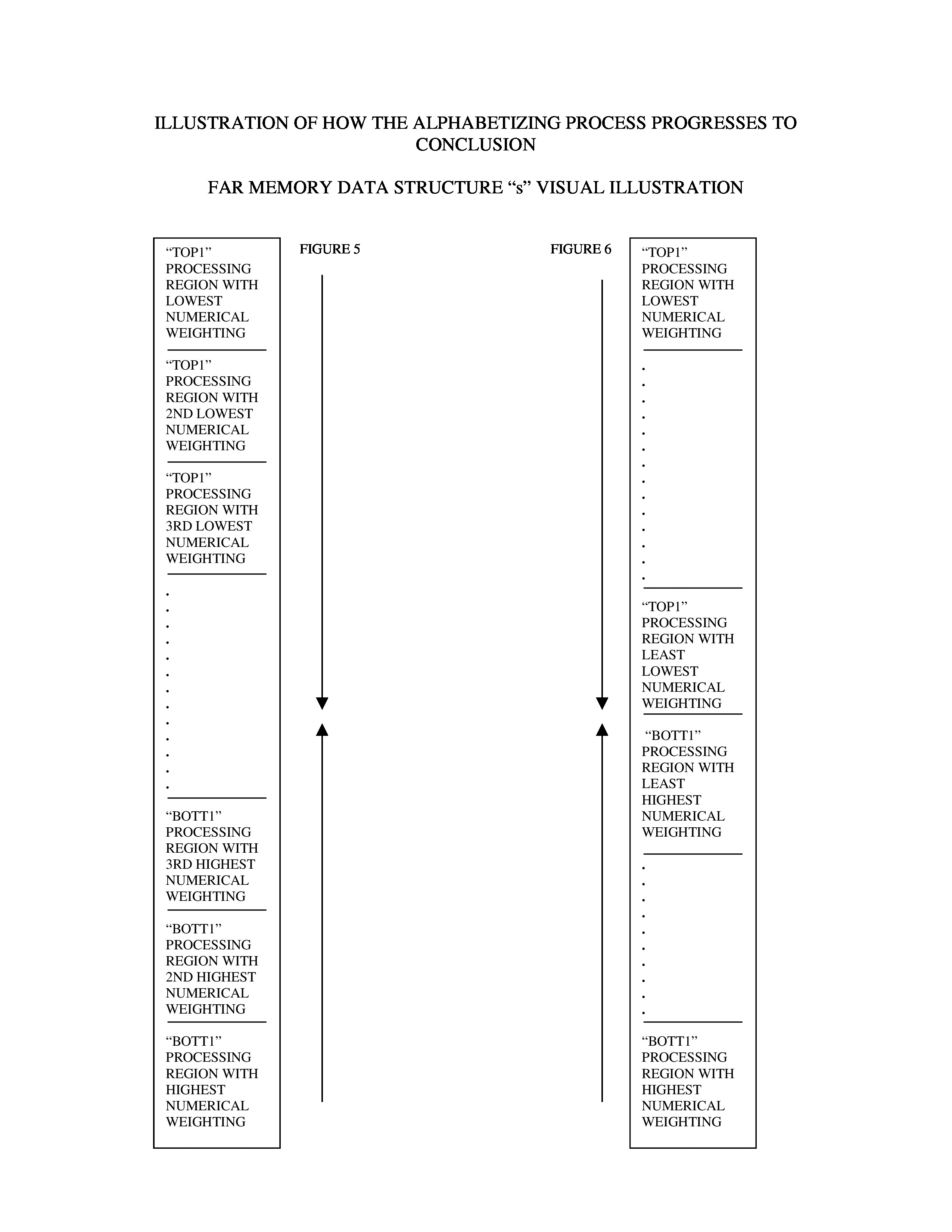
Both processing regions will approach each other in spatial proximity as they move toward the center of the far memory data structure “s” from being redefined with each pass through the “main” processing loop. Each new “top1” processing region will have a higher numerical weight than its predecessor “top1” region. Each new “bott1” processing region will have a lower numerical weight than its predecessor “bott1” region. Please refer to figures 3, 4, 5, and 6 for a visual illustration of the progression of the algorithm as successive “top1” and “bott1” processing regions are redefined with each pass through the “main” processing loop.
Notice what happens in Figure 6 after the processing in successive “top1” and “bott1” processing regions reaches the middle of far memory in the far memory data structure “s”. The “top1” processing region with the least lowest numerical weight is adjacent to the “bott1” processing region with the least highest numerical weight. The processing will cease at this point because there will be no more items left to sort. The “main” processing loop will then be exited and the new sorted array of item positions stored in far memory data structure “s1” will be written to a new data file. (See Figures 9 and 10).
Here, I want to talk about ways the “main” processing loop could be exited before the data is written back to a newly sorted data file. As the processing draws to a close in the middle of the far memory data structure “s”, it will not necessarily end with an even pair of final “top1” and “bott1” processing regions. It can also near completion with either of the “top1” or “bott1” processing regions having its “main” processing loop exit variable set to attempt to exit the “main” processing loop. To be more specific, the “top1” processing region could have its “main” loop exit variable “qqq” set to 1, which means there are no more “top1” regions to be redefined. The “bott1” processing region could have its “main” loop exit variable “sss” set to 0, meaning there is another “bott1” processing region to be redefined and sorted. The opposite of this can also occur.
AN ANALOGY THAT MAY HELP CLARIFY THE LOGIC FLOW
Knowing this narrative may be overwhelming for some readers, I would like to take a page from American history that may be helpful in creating a better understanding of how my algorithm works.
During the latter part of the 19th century, the United States turned its attention to nation building. Connecting the vast expanse of North America by way of a coast-to-coast railroad became a national priority. This was the start of America’s first Transcontinental Railroad.
Two railroad companies, the Union Pacific and the Central Pacific, spearheaded this ambitious and daunting task. The Central Pacific began building its railway eastward from Sacramento, California, while the Union Pacific began construction work heading westward from Omaha, Nebraska.
Both crews in the east and west worked relentlessly for seven years. On April 28, 1868 the Union Pacific’s construction gang of Chinese and Irish workers laid ten miles of railroad track in a single day as a result of a $10,000 bet that it could actually be done. On May 10, 1869 the construction was completed at Promontory Point in the Utah territory. The Union Pacific’s No. 119 engine and the Central Pacific’s No. 60 engine, Jupiter, were drawn up face-to-face separated by the width of a single railroad tie. At the Golden Spike ceremony, three spikes were driven in to connect the two railways: gold, silver and a composite spike made from gold, silver and iron. Travel time between the east and west coasts of the United States was reduced from 4 to 6 months to only 6 days by railroad!
Now, the progression of my algorithm is quite similar to the construction of America’s first Transcontinental Railroad when you take a moment to really think about it. As the algorithm moves along, it begins to resemble two work crews gradually progressing towards a conclusion in the middle of the allocated far memory space, which is like a long stretch of terrain awaiting the arrival of “sorting construction labor”, so to speak. The “top1” and “bott1” processing regions are like “two construction gangs” that commence “sorting work” that begins at opposite ends of the allocated memory space. They each work hard to sort items of the same numerical weight as previously described, while constantaly moving closer and closer to one another. After the program loops around the “main” processing loop and new “top1” and “bott1” processing regions have been defined, the process repeats itself. Finally, The “Golden Spike Ceremony” occurs when the “top1” and “bott1” processing regions are adjacent to one another somewhere near the middle of the allocated far memory segment - Promontory Point in the Utah territory, if I may use that to hopefully foster a better understanding of my algorithm.
A POTENTIAL PROBLEM AND A REMEDY
Here, I would like to expand on a potential problem with my algorithm and a recommended solution that should take care of it. The 2 dimensional “grid” conventional data structure is used extensively to manipulate items in the “top1” and “bott1” processing regions. It is designed to hold up to 150 items of the same numerical weight. You need to be conscious about how much row depth you give the 2 dimensional “grid” conventional data structure so it and other conventional data structures taken together don’t breach the 64K data segment of the small memory model that is used. The problem arises if there are more than 150 items in a “top1” or “bott1” processing region. The algorithm won’t abort or malfunction, but rather it will include only the first 150 items in a processing region. I never really tried to address this potential snafu, because it is highly unlikely to occur in the first place. There would have to be more than 150 “Smiths” or “Joneses” to trigger the glitch. This could potentially happen in a voter registration verification data file that could include a large number of same last names.
A good way to correct this is to declare a fourth far memory data structure of the same size as each of the first 3. It would replace and perform the job of the 2 dimensional “grid” conventional data structure, yet it would always be large enough to hold all the items for a particular numerical weight. This is because it would be allocated to hold as many items as are in the entire data file.
JUST SAY “NO” TO REDUNDANT, SPEED ROBBING CODE
Many of you may be wondering by now about the speed of the algorithm. I tested it with a binary fixed record width text file containing 10,959 part numbers. On a Gateway Pentium 4 tower CPU using an old 6 GB Quantum Bigfoot hard drive the processing took a little over 3 seconds. When it was run on a Dell M5030 laptop with an AMD V160 Processor at 2.4 GHz it took about 1 second. There are some areas in the “do-while” loop processing that could be redesigned or eliminated that should further increase the processing speed since less work is required to achieve the same result. After I finished this in 1996 it seemed to work in a reasonable amount of time so I didn’t go back and try to optimize it some more. Here I will elaborate with some selected areas in the code that could be improved to yield more processing speed.
|
|
This block of code that tests for ASCII characters 32 through 126 could be replaced with the C++ function, “atoi()”. It would eliminate much of the repetitive conditional “if-then” logic structure comparisons and convert the character to an integer. This new integer value could then be used in the math formula that computes numerical weights for each item. Here is another place for adding some speed:
|
|
In the “top1” and “bott1” processing sections of the code, there is a patch of code enclosed by processing loop “2”. There are two places where the “far_memory_contents_2” file stream position offset is calculated twice. It is then used to retrieve data into the “name” conventional data structure for comparison operations in two different rows in the 2 dimensional “grid” conventional data structure. It only needs to be calculated once to achieve the same result. In fact, the “name” conventional data structure only needs to retrieve the data once with each processing loop “2” loop instead of twice.
CONCLUSION
I have used this sorting algorithm in many C++ applications, typically for sorting part numbers or customer names that are to be previewed as reports. It has proven itself to be reliable as well as fast. I have also adapted it for sorting numbers and dates. If you would like to learn more about my developer skills, then please visit my software developer website. Additionally, be sure to check out my computer repair services and my "fix my computer" technical tips.
References:
http://www (dot) accelerationwatch (dot) com/promontorypoint (dot) html
http://en (dot) wikipedia (dot) org/wiki/Promontory,_Utah
http://www (dot) history (dot) com/topics/transcontinental-railroad